If you want to create a deep learning model using the PyTorch or TensorFlow libraries, you might encounter some difficulties in your learning journey. Although they provide highly efficient, optimized code, this comes at the cost of abstracting a lot of the underlying mechanisms. Fortunately, in this article, we will build an artificial neuron from scratch to provide a deeper understanding of how a neuron works.
Table of contents
Open Table of contents
Understanding Neurons with a Puzzle
You may have seen a puzzle on the Internet that looks like this:
| Input | Output |
|---|---|
| 11 | 23 |
| 23 | 47 |
| 36 | 73 |
| 49 | 99 |
| 55 | ?? |
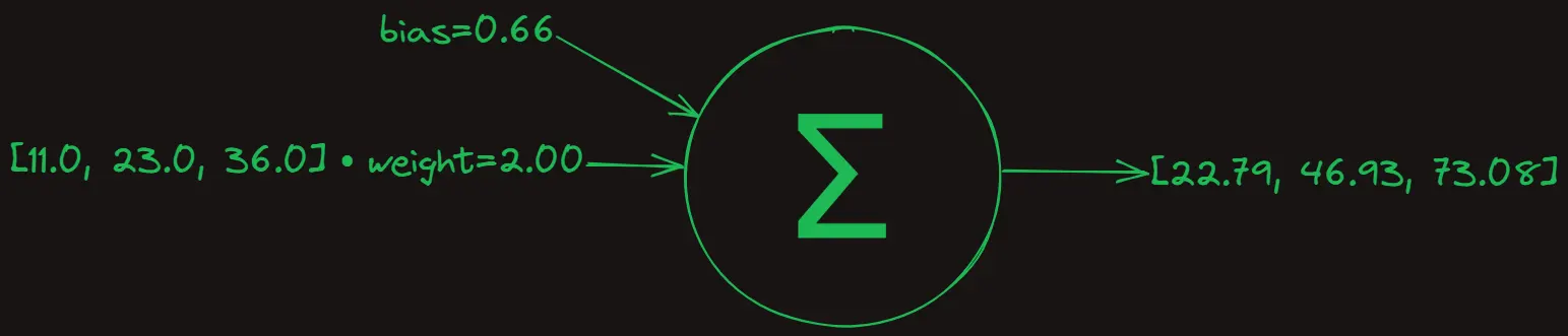
Spoiler alert: the answer is 111! How do I know? Well, because I created this puzzle. It’s based on a linear equation 2x+1. However, we can use the smallest component in a neural network, a neuron, to figure out the answer!
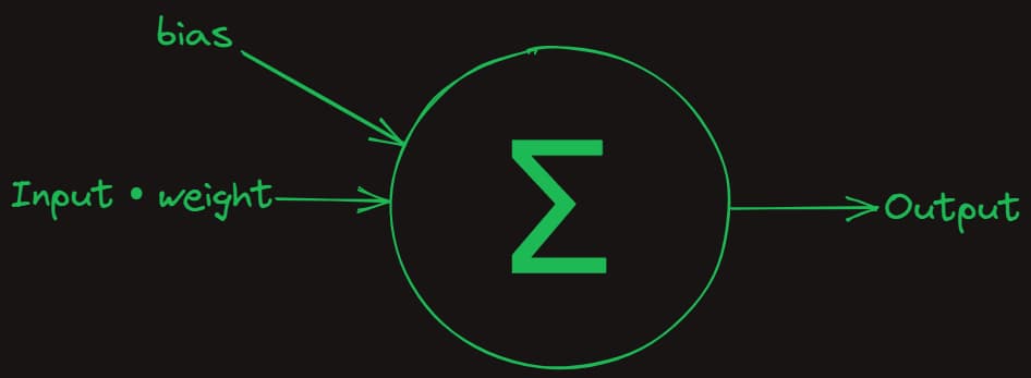
A neuron, also known as a perceptron, is a mathematical function that takes an input, x, performs calculations, and returns an output, y. For example, when x=11, the neuron calculation yields y=23.
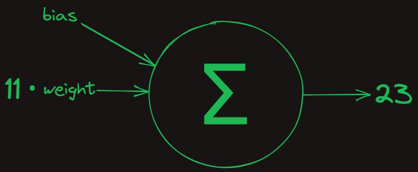
As can be seen in the diagram above, the components of a neuron are weight and bias. The weight is multiplied with the input (in this case, x=11), then the result is added to the bias. So, to correctly solve our puzzle, the weight and bias must be set to 2 and 1, respectively. This signifies that the weight and bias represent the linear function 2x+1.
So, how do we determine the values for weight and bias? Essentially, we need to create a learning mechanism that allows weight and bias to find thier correct values.
Training a Neuron
Step one: Initializing weight and bias
We initialize weight and bias (also called parameters) at arbitrary values. For instance, we could set weight=0.1 and bias=0.6.
weight = 0.1
bias   = 0.6
Step two: Pass the inputs through the neuron
This step involves passing the inputs through the neuron to get the output. In machine learning, this step is known as forward propagation.
We use Numpy library, a Python library for scientific computing, to perform the calculations.
import numpy as np
x_train = np.array([11.0, 23.0, 36.0, 49.0])
y_prediction = np.dot(x_train, weight) + bias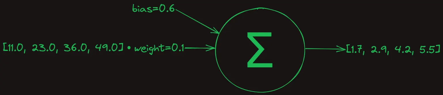
From the above results, it’s clear that our predictions are far from accurate. For example, when x=11, we predict y=1.7, when the correct output should be y=23. So, how do we adjust the weight and bias to correct this? A logical approach would be to calculate the difference between the predicted output and the actual output, then adjust the weight and bias based on this difference.
Step three: Calculating the Error
Here we calculate the difference between the predicted and actual values. This is known as loss function in machine learning, and our goal is to minimize the values produced by this function.
y_train = np.array([23.0, 47.0, 73.0, 99.0])
loss = y_train - y_prediction  # [21.3, 44.1, 68.8, 93.5]
To adjust weight and bias, we can employ a method called gradient descent, which helps us find the optimal values for weight and bias.
Step four: Calculating the gradients
Step four involves calculating the gradients, which represent the direction and rate of change of the loss function with respect to the parameters. We use the chain rule of calculus to compute these gradients. This step is known as backward propagation, as it involves adjusting the parameters of the neuron.
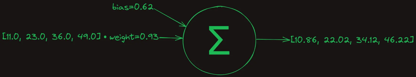
derivative_weight = -1 * np.dot(x_train, loss) # -8306.9
derivative_bias = -1 * np.sum(loss) # -227.7
Next, we update the weight and bias values. However, gradient descent tells us in which direction to adjust our values, not what the actual values for weight and bias should be. To approach the target values slowly and avoid overshooting, we use a small learning rate to multiply with the derivative.
learning_rate = 0.0001
weight -= learning_rate * derivative_weight # 0.93
bias -= learning_rate * derivative_bias # 0.62
Testing the Neuron
The results are promising! The weight has increased from 0.1 to 0.93, while the bias has slightly increased from 0.6 to 0.62.
Let’s now examine the code:
import numpy as np

x_train = np.array([11.0, 23.0, 36.0, 49.0])
y_train = np.array([23.0, 47.0, 73.0, 99.0])

weight = 0.1
bias = 0.6
learning_rate = 0.0001

y_prediction = np.dot(x_train, weight) + bias

loss = y_train - y_prediction

derivative_weight = -1 * np.dot(x_train, loss)
derivative_bias = -1 * np.sum(loss)

weight -= learning_rate * derivative_weight
bias -= learning_rate * derivative_bias
Now that we have completed our first iteration of neuron training, let’s run another iteration and see what result we get.
Definitely an improvement! As you can observe, the results are increasingly approximating the actual values. However, it appears that the neuron requires several iterations before it converges.
Let’s run the neuron for 50 iterations, as demonstrated in the code below:
import numpy as np

x_test = np.array(55.0)
x_train = np.array([11.0, 23.0, 36.0, 49.0])
y_train = np.array([23.0, 47.0, 73.0, 99.0])

weight = 0.1
bias = 0.6
learning_rate = 0.0001

for step in range(50):
  y_prediction = np.dot(x_train, weight) + bias

  loss = y_train - y_prediction

  derivative_weight = -1 * np.dot(x_train, loss)
  derivative_bias = -1 * np.sum(loss)

  weight -= learning_rate * derivative_weight
  bias -= learning_rate * derivative_bias

  if step % 10 == 0:
    print(f"Step {step}, Answer: {np.dot(x_test, weight) + bias}")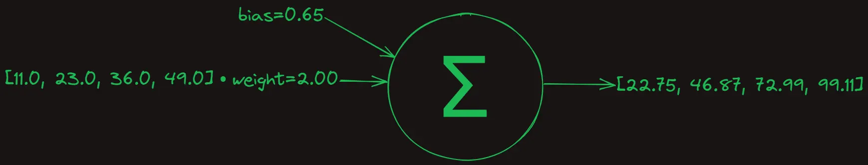
Step 0, Answer: 51.81072
Step 10, Answer: 110.97905835174222
Step 20, Answer: 111.17498229579553
Step 30, Answer: 111.17550167919178
Step 40, Answer: 111.17537368728773
Here we introduce x_test=55, the input we have been seeking in this puzzle! We have now obtained a result, which appears to be 111. However, how can we confirm the accuracy of our answer? What if the neuron is producing wrong results? To address this concern, we can divide our input data as illustrated in the code below:
import numpy as np

x_test = np.array(49.0)
x_train = np.array([11.0, 23.0, 36.0])
y_train = np.array([23.0, 47.0, 73.0])

weight = 0.1
bias = 0.6
learning_rate = 0.0001

for step in range(50):
  y_prediction = np.dot(x_train, weight) + bias

  loss = y_train - y_prediction

  derivative_weight = -1 * np.dot(x_train, loss)
  derivative_bias = -1 * np.sum(loss)

  weight -= learning_rate * derivative_weight
  bias -= learning_rate * derivative_bias

  if step % 10 == 0:
    print(f"Step {step}, Answer: {np.dot(x_test, weight) + bias}")
In the code above, we took the last element, 49, from x_train and instead put it in y_test. We use it as a validation set. We did this because it allows us to verify the accuracy of our neuron’s output. We can confidently do this as we know that the correct output for 49 is indeed 99.
Step 0, Answer: 23.767879999999998
Step 10, Answer: 90.61052067032544
Step 20, Answer: 98.26305744118851
Step 30, Answer: 99.13906937817997
Step 40, Answer: 99.23925422441026
Now we can pass the value 55 into the neuron!
puzzle_prediction = np.dot(np.array(55.0), weight) + bias
print(puzzle_prediction) # 111.32
We can also validate this by manually calculating it using the equation: 2 * 55.0 + 1, which equals 111. Do you want to get a result closer to 111, rather than 111.32? Consider training the neuron for additional iterations.
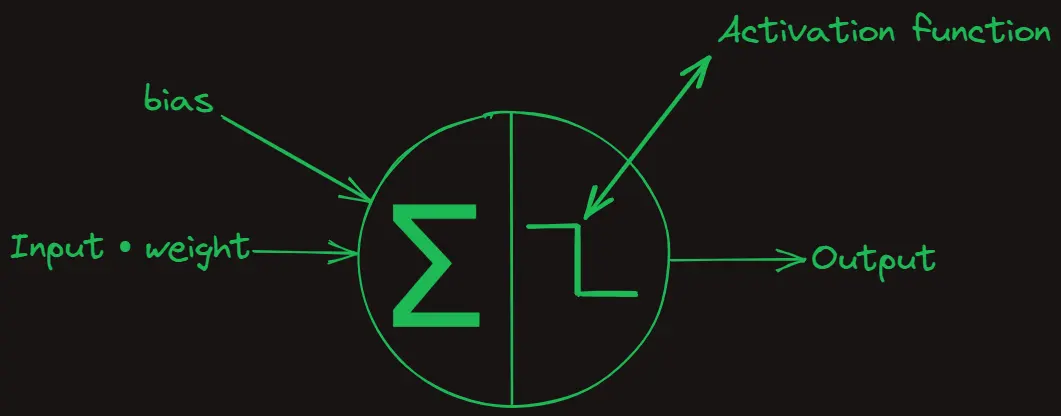
We have successfully solved the puzzle with the power of neurons. That being said, the neuron we trained essentially represents a linear regression model. This means that it cannot learn non-linear equations. For instance, it cannot solve a cubic polynomial such as x^3 + 2x + 1 using just one neuron, because a single weight and bias can’t fit the equation. To address this, we would need a activation function, such as the Rectified Linear Unit (ReLU), which introduces non-linearity.
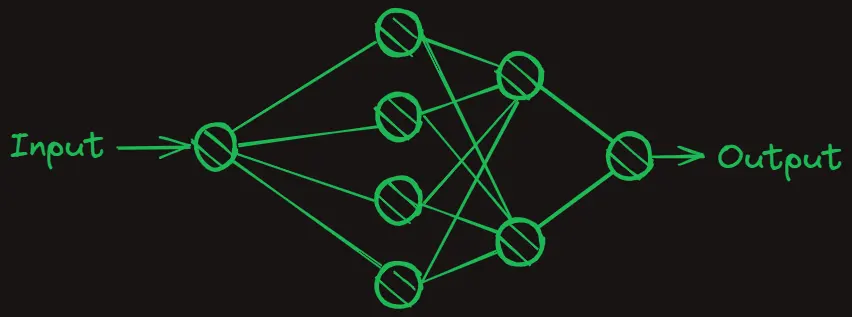
Furthermore, to learn complex representations, we might need many neurons stacked in multiple layers. This structure is known as a neural network, and it’s ubiquitous in modern machine learning applications, such as large language and diffusion models. At their core, these networks are simply composed of neurons with learnable weights and biases.
Conclusion
In this article, we explored how a neuron functions by solving a numerical sequence puzzle. We dived into the inner workings and experienced how weight and bias operate in action.